ヒストグラムの統計結果hの分割点はh$breaks、密度はh$densityに入っている。 分割点の数は密度よりも一つ多い。
stepfun()を用いると簡単。\((x_1, x_2, \dots, x_n)\)よりも\((y_0, y_1, \dots, y_n)\)が一つ多いことに注意。既定では区間\([x_{i}, x_{i+1}]\)の一定値\(c_i = (1 - f)y_i + fy_{i+1}\)なので、区間の右の重み\(f\)を0にすると\(x_i\)に\(y_i\)が使われる。
n <- 1000
m <- 5
dof <- m - 1
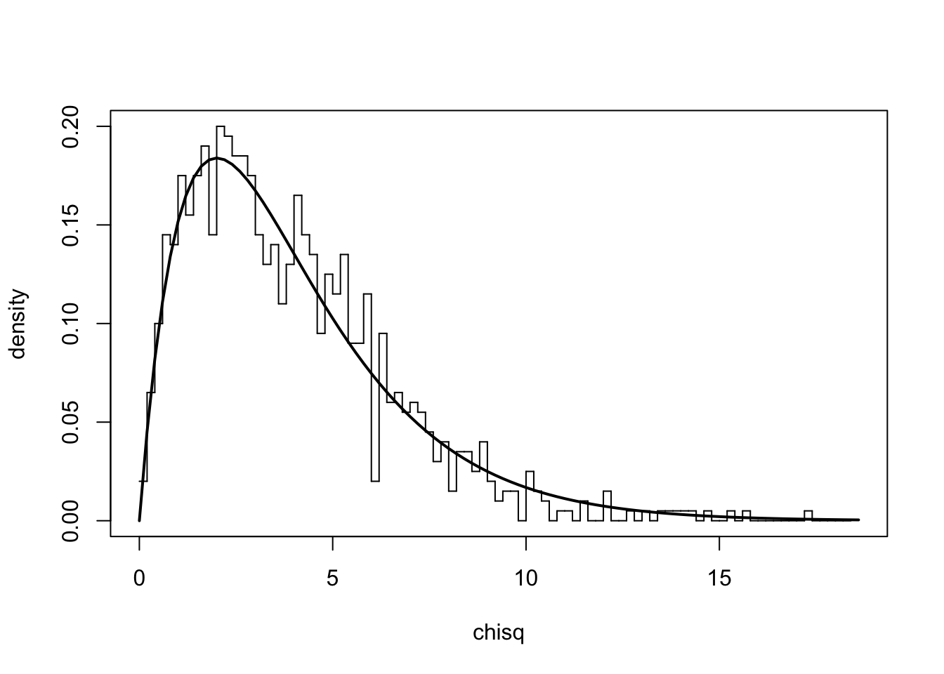
chisq <- rchisq(n, dof)
h <- hist(chisq, breaks = 100, plot = FALSE)
plot(h$breaks, dchisq(h$breaks, dof), type = "l", lwd = 2, xlab = "chisq", ylab = "density", ylim = c(0, max(h$density)))
lines(stepfun(h$breaks, c(NA, h$density, NA), f = 0), do.points = FALSE)
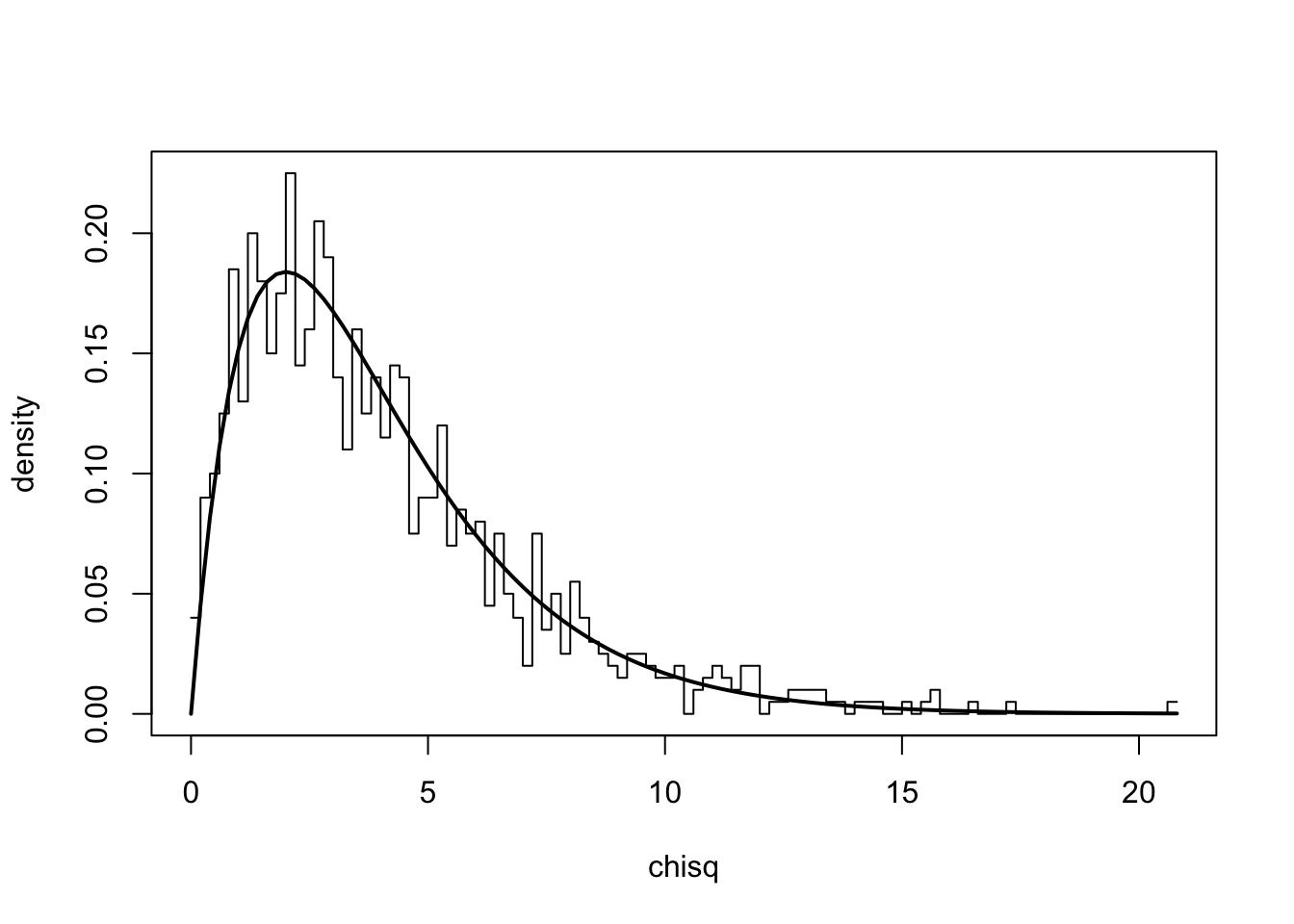
stepfun()を使わない方法。折れ線を描くために、分割点は最初の点と最後の点の間の要素を値を、密度は全体を複製する。
n <- 1000
m <- 5
dof <- m - 1
chisq <- rchisq(n, dof)
h <- hist(chisq, breaks = 100, plot = FALSE)
plot(c(h$breaks[1], rep(h$breaks[2:(length(h$breaks)-1)], each = 2),
       h$breaks[length(h$breaks)]), rep(h$density, each = 2),
  xlab = "chisq", ylab = "density", type="l")
lines(h$breaks, dchisq(h$breaks, dof), lw = 2)