制約付き数値最適化

optimization

package

nloptr

Author

榎本剛

Published

June 30, 2025

nloptはCで書かれた非線型最適化ライブラリで、さまざまな言語から使うことができる。 Rのパッケージはnloptrで、nloptは別物である。

インストール

まず、ライブラリをインストールする。 CコンパイラとCMakeが必要。ソースを展開したら、その中でbuildディレクトリを作り、cmakeを実行し、makeからコンパイル、インストールを指示する。インストール先として~/.localを指定し、Pythonのインターフェースも構築する例を示す。MacPortsで入れたPython (python313など)をsudo port select python python313してあり、/opt/local/bin/pythonというシンボリックリンクがあることを想定している。 PythonインターフェースはRから使うには不要である。

% cmake .. -DDCMAKE_INSTALL_PREFIX=${HOME}/.local -DPython_EXECUTABLE=/opt/local/bin/python
% make
% make install

Rのインターフェースを構築する際には、pkg-configが用いられるので、確認しておく。なお、MacPortsのパッケージ名はハイフンのないpkgconfigである。

% pkg-config --libs nlopt

あとはinstall.packages("nloptr")をRのコンソールで実行してパッケージをインストールするだけである。

制約なし最適化

VignettesにあるRosenbrock函数の最適化を試してみよう。

library(nloptr)

eval_f <- function(x) {
  100 * (x[2] - x[1] * x[1])^2 + (1 - x[1])^2
}

eval_grad_f <- function(x) {
  c(-400 * x[1] * (x[2] - x[1] * x[1]) - 2 * (1 - x[1]), 200 * (x[2] - x[1] * x[1]))
}

x0 <- c(-1.2, 1)

opts <- list("algorithm" = "NLOPT_LD_LBFGS", "xtol_rel" = 1.0e-8)

res <- nloptr(x0 = x0,
              eval_f = eval_f,
              eval_grad_f = eval_grad_f,
              opts = opts)
res


Call:
nloptr(x0 = x0, eval_f = eval_f, eval_grad_f = eval_grad_f, opts = opts)



Minimization using NLopt version 2.10.0 

NLopt solver status: 1 ( NLOPT_SUCCESS: Generic success return value. )

Number of Iterations....: 56 
Termination conditions:  xtol_rel: 1e-08 
Number of inequality constraints:  0 
Number of equality constraints:    0 
Optimal value of objective function:  7.35727226897802e-23 
Optimal value of controls: 1 1

56ステップで収束した。コスト函数と勾配の共通部分の計算を節約するために、二つをまとめることもできる。

eval_f_list <- function(x) {
  f1 <- x[2] - x[1] * x[1]
  f2 <- 1 - x[1]
  list(
    "objective" = 100 * f1^2 + f2^2,
    "gradient" = c(-400 * x[1] * f1 - 2 * f2, 200 * f1))
}

res <- nloptr(x0 = x0,
              eval_f = eval_f_list,
              opts = opts)
res


Call:
nloptr(x0 = x0, eval_f = eval_f_list, opts = opts)


Minimization using NLopt version 2.10.0 

NLopt solver status: 1 ( NLOPT_SUCCESS: Generic success return value. )

Number of Iterations....: 56 
Termination conditions:  xtol_rel: 1e-08 
Number of inequality constraints:  0 
Number of equality constraints:    0 
Optimal value of objective function:  7.35727226897802e-23 
Optimal value of controls: 1 1

制約あり最適化

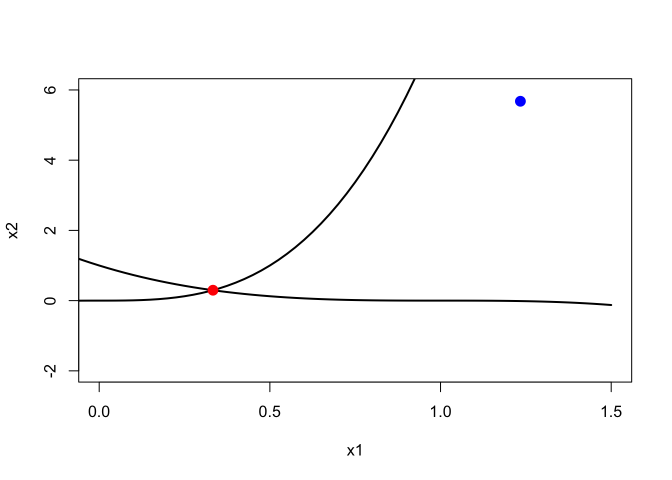
次の制約あり最適化問題を考える。

\[ \min_{x \in \mathbb{R}^n}\sqrt{x_2} \] \[ \begin{aligned} \text{s.t.}\;x_2 &\ge 0\\ x_2 &\ge (a_1x_1 + b_1)^3\\ x_2 &\ge (a_2x_1 + b_2)^3 \end{aligned} \]

ここで、\(a_1 = 2,\,b_1 = 0,\,a_2 = -1,\,b_2 = 1\)である。制約条件は \(g(x)\le 0\) という形に書き換える。

\[ \begin{aligned} (a_1x_1 + b_1)^3 - x_2 &\le 0\\ (a_2x_1 + b_2)^3 - x_2 &\le 0 \end{aligned} \]

勾配を用いる制約あり最適化はNLOPT_LD_MMA、NLOPT_LD_CCSAQ、NLOPT_LD_SLSQPが使える。この中でNLOPT_LD_SLSQPのみ非線型の制約を課すことができる。マニュアルではNLOPT_LD_CCSAQをまず試すことを勧めている。この例では、NLOPT_LD_MMAが最も少ない21回で収束した。 NLOPT_LD_CCSAQは24回、NLOPT_LD_SLSQPは43回必要だった。

eval_f0 <- function(x, a, b) {
  sqrt(x[2])
}

eval_grad_f0 <- function(x, a, b) {
  c(0, 0.5 / sqrt(x[2]))
}

eval_g0 <- function(x, a, b) {
  (a * x[1] + b)^3 - x[2]
}

eval_jac_g0 <- function(x, a, b) {
  rbind(c(3 * a[1] * (a[1] * x[1] + b[1])^2, -1.0),
        c(3 * a[2] * (a[2] * x[1] + b[2])^2, -1.0))
}
a <- c(2, -1)
b <- c(0, 1)

opts = list(
  "algorithm" = "NLOPT_LD_MMA",
  "xtol_rel" = 1.0e-8,
  "print_level" = 2,
  "check_derivatives" = TRUE,
  "check_derivatives_print" = "errors"
)

res0 <- nloptr(x0 = c(1.234, 5.678),
               eval_f = eval_f0,
               eval_grad_f = eval_grad_f0,
               lb = c(-Inf, 0), ub = c(Inf, Inf),
               eval_g_ineq = eval_g0,
               eval_jac_g_ineq = eval_jac_g0,
               opts = opts, a = a, b = b)

Checking gradients of objective function.

Derivative checker results: 0 error(s) detected.

Checking gradients of inequality constraints.

Derivative checker results: 0 error(s) detected.

iteration: 1
    f(x) = 2.382855
    g(x) = (9.354647, -5.690813)
iteration: 2
    f(x) = 2.356135
    g(x) = (-0.122988, -5.549587)
iteration: 3
    f(x) = 2.245864
    g(x) = (-0.531886, -5.038655)
iteration: 4
    f(x) = 2.019102
    g(x) = (-3.225103, -3.931195)
iteration: 5
    f(x) = 1.740934
    g(x) = (-2.676263, -2.761136)
iteration: 6
    f(x) = 1.404206
    g(x) = (-1.674055, -1.676216)
iteration: 7
    f(x) = 1.022295
    g(x) = (-0.748790, -0.748792)
iteration: 8
    f(x) = 0.685203
    g(x) = (-0.173206, -0.173207)
iteration: 9
    f(x) = 0.552985
    g(x) = (-0.009496, -0.009496)
iteration: 10
    f(x) = 0.544354
    g(x) = (-0.000025, -0.000025)
iteration: 11
    f(x) = 0.544331
    g(x) = (0.000000, 0.000000)
iteration: 12
    f(x) = 0.544331
    g(x) = (-0.000000, 0.000000)
iteration: 13
    f(x) = 0.544331
    g(x) = (-0.000000, 0.000000)
iteration: 14
    f(x) = 0.544331
    g(x) = (-0.000000, 0.000000)
iteration: 15
    f(x) = 0.544331
    g(x) = (-0.000000, 0.000000)
iteration: 16
    f(x) = 0.544331
    g(x) = (-0.000000, 0.000000)
iteration: 17
    f(x) = 0.544331
    g(x) = (-0.000000, 0.000000)
iteration: 18
    f(x) = 0.544331
    g(x) = (-0.000000, 0.000000)
iteration: 19
    f(x) = 0.544331
    g(x) = (0.000000, 0.000000)
iteration: 20
    f(x) = 0.544331
    g(x) = (-0.000000, -0.000000)
iteration: 21
    f(x) = 0.544331
    g(x) = (0.000000, 0.000000)

x1 <- seq(-1, 1.5, length.out = 101)
plot(x1, (a[1] * x1 + b[1])^3, type = "l", lwd = 2,
     xlim = c(0, 1.5), ylim = c(-2, 6),
     xlab = "x1", ylab = "x2")
lines(x1, (a[2] * x1 + b[2])^3, lwd = 2)
points(res0$x0[1], res0$x0[2], cex = 1.5, pch = 16, col = "blue")
points(res0$solution[1], res0$solution[2], cex = 1.5, pch = 16, col = "red")