bfgs <- function(par, fn, gr, ..., control){
  control <- modifyList(list(
    maxit = 100, debug = FALSE,
    ctol = 1e-10, gtol = 1e-7, stol = 1e-7), control)
 if (control$debug)  print(control)

  n <- length(par)
  H <- diag(n)
  g <- gr(par, ...)
  alpha <- min(1, 1. / sum(abs(g)))
  new_par <- par - alpha * g
  s <- -alpha * g
  y <- gr(new_par, ...) - g
  ys <- sum(y * s)
  H <- ys / sum(y * y) * diag(n)
  if (control$debug) cat("Initial Hessian:", H, "\n")

  cost <- rep(0, control$maxit + 1)
  gnorm.hist <- rep(0, control$maxit + 1)
  par.hist <- matrix(0, nrow = control$maxit + 1, ncol = n)

  for (iter in seq_len(control$maxit)) {
    cost[iter] <- fn(par, ...)

    gnorm <- sqrt(sum(g^2))
    gnorm.hist[iter] <- gnorm
    par.hist[iter, ] <- par

    if (control$debug) cat("Iteration:", iter, "Cost:", cost[iter], "Gradient Norm:", gnorm, "\n")
    if (gnorm < control$gtol) {
      convergence <- 0
      break
    }
    if (max(abs(s)) < control$stol) {
      convergence <- 1
      break
    }

    new_par <- par - drop(H %*% g)
    s <- new_par - par
    new_gr <- gr(new_par, ...)
    y <- new_gr - g
    ys <- sum(y * s)
    if (ys > control$ctol) {
      rho <- 1 / ys
      H <- (diag(n) - rho * outer(s, y)) %*% H %*% (diag(n) - rho * outer(y, s)) + rho * outer(s, s)
      if (control$debug)  cat("Updated Hessian:", H, "\n")
    } else {
      H <- ys / sum(y * y) * diag(n)
      if (control$debug)  cat("Reset Hessian:", H, "\n")
    }
    if (iter == control$maxit) {
      convergence <- 2
    }

    par <- new_par
    g <- new_gr
  }

  list(par = par.hist[1:iter, ], convergence = convergence,
       cost = cost[1:iter], gnorm = gnorm.hist[1:iter])
}BFGS
DA
ML
optimization
準ニュートン法による数値最適化
数値最適化はデータ同化や機械学習などで、データから最適解を求めるための数値手法である。
函数\(f(\mathbf{x})\)が最小になるような\(\mathbf{x}\)を求める問題を考える。 \(\mathbf{x}\)は制御変数と呼ばれ、初期値を推定するデータ同化では自由度\(n\)の場を表す。 \(\mathbf{x}\)の近傍で\(f(\mathbf{x})\)が二次に近いと仮定し、 \(\mathbf{x}\)から\(\mathbf{d}\)だけ変化させた\(f(\mathbf{x}+ \mathbf{d})\)をテーラー展開で二次まで近似する。
\[ f(\mathbf{x} + \mathbf{d}) \approx f(\mathbf{x}) +\mathbf{g}^\mathrm{T}\mathbf{d} + \mathbf{d}^\mathrm{T}\mathbf{G}\mathbf{d} \]
ここで、\(\mathbf{g} = \nabla f(\mathbf{x})\)は勾配、\(\mathbf{G} = \nabla^2 f(\mathbf{x})\)はヘシアンである。
代表的な準ニュートン法であるBFGS法 (Broyden 1970; Fletcher 1970; Goldfarb 1970; Shanno 1970)は、へシアン逆行列\(\mathbf{H}_k\)を明示的に計算することなく、曲率についての情報を函数値や勾配から構築し、反復の中で以下のBFGS公式に基づいて更新する (Nocedal and Stephen J. Wright 2006)。
\[ \mathbf{H}_{k+1} = \mathbf{V}_k^\mathrm{T}\mathbf{H}_k\mathbf{V}_k + \rho_k\mathbf{s}_k\mathbf{s}_k^\mathrm{T} \tag{1}\]
ここで、\(k\)は反復の番号、\(\mathbf{s}_k = \mathbf{x}_{k+1} - \mathbf{x}_k\)、\(\mathbf{y}_k = \nabla f_{k+1} - \nabla f_k\)、\(\mathbf{V}_k = \mathbf{I} - \rho_k\mathbf{y}_k \mathbf{s}_k^\mathrm{T}\)及び\(\rho_k = 1/\mathbf{y}_k^\mathrm{T}\mathbf{s}_k\)である。
二次函数の仮定の下では、ステップ幅はおよそ1なので、ステップ幅計算は省略することもできる。 BFGSには、ヘシアン逆行列を明示的に保存せずに、過去のステップと勾配から行列ベクトル積\(\mathbf{G}^{-1}\mathbf{g}\)を更新するメモリ節約版もあるが、ここではモデルの自由度が小さい場合を考え、ヘシアン逆行列を明示的に保存する。
BFGSはR標準の{stat}のoptim(method = "BFGS")に実装されている。 その他いくつかのパッケージで使える(Taskview Optimization参照)。 パッケージの最適化手法で、最適化中のコスト函数や勾配ノルムの履歴を出力するには、ログをテキスト処理するか、大域変数に記録する。 捕食・被食モデルでは、組込の optim() を使い、後者の方法で履歴を保存した例を示している。
ここでは、BFGS更新Equation 1を実装したコードを示す。
\(\mathbf{s}_k\)と\(\mathbf{y}_k\)は二つの反復回の差なので、\(k=0\)では勾配からステップ幅を計算する。 ヘシアン逆行列\(\mathbf{H}\)は次のように初期化する。
\[ \mathbf{H} = \frac{\mathbf{s}^\mathrm{T}\mathbf{y}}{\mathbf{y}^\mathrm{T}\mathbf{y}}\mathbf{I} \] ここで、\(\alpha = 1/\sum_j|g_j|,\,j = 1, \dots, n\)、\(\mathbf{s} = -\alpha\mathbf{g}_0\)、\(\mathbf{y} = \mathbf{g}(\mathbf{x}_0-\alpha\mathbf{g}_0) - \mathbf{g}(\mathbf{x}_0)\)である。
Rosenbrock函数
\[ f(x, y) = (1 - x)^2 + 100(y - x^2)^2 \] を\((-1.2, 1)\)から最小化してみよう。
rosen <- function(x, y) {
  (1 - x)^2 + 100 * (y - x^2)^2
}

rosen.gr <- function(x, y) {
  c(-2 * (1 - x) - 400 * x * (y - x^2), 200 * (y - x^2))
}

rosen.bfgs <- function(par, control = list()) {
  control <- modifyList(list(maxit = 100, gtol = 1e-6), control)

  bfgs(par,
       function(w){rosen(w[1], w[2])},
       function(w){rosen.gr(w[1], w[2])}, control = control)
}

result <- rosen.bfgs(c(-1.2, 1), control = list(maxit = 100, gtol = 1e-7))
コスト函数は8ステップまで減少しているが、その後乱高下し、13ステップ目で大きく低下し、その後の変化は小さい。
par(mar = c(4, 5, 2, 2))
plot(1:length(result$cost), log10(result$cost), type="b", pch=19, cex=2, lwd=2,
     xlab="iteration", ylab="log10(cost)", main="Rosenbrock BFGS",
     cex.main=2, cex.axis=2, cex.lab=2)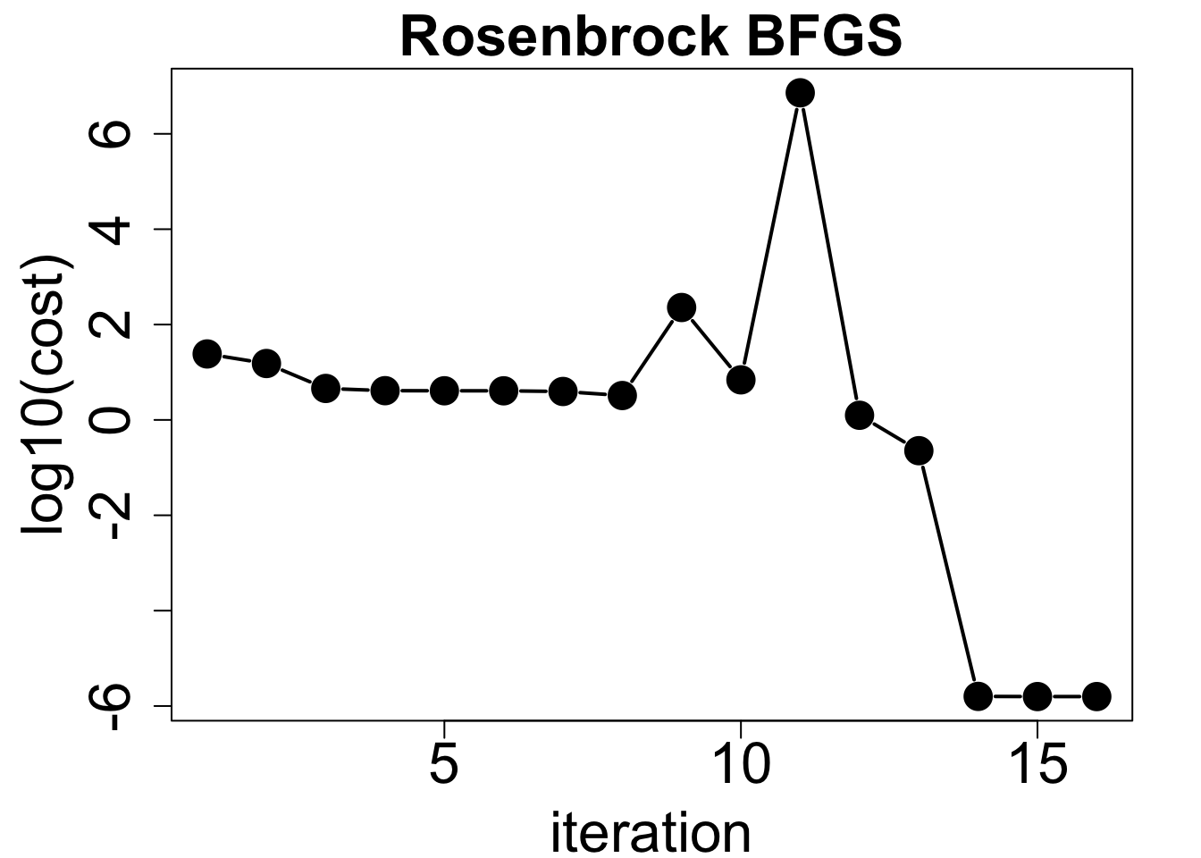
一方、勾配ノルムは5ステップ目まで減少し、その後上昇に転じる。 11ステップ目で急増するが、その後大きく減少する。 最終的な勾配ノルムは閾値\(1 \times 10^{-7}\)よりも大きい。
par(mar = c(4, 5, 2, 2))
plot(1:length(result$cost), log10(result$gnorm), type="b", pch=19, cex=2, lwd=2,
     xlab="iteration", ylab="log10 |g|", main="Rosenbrock BFGS",
     cex.main=2, cex.axis=2, cex.lab=2)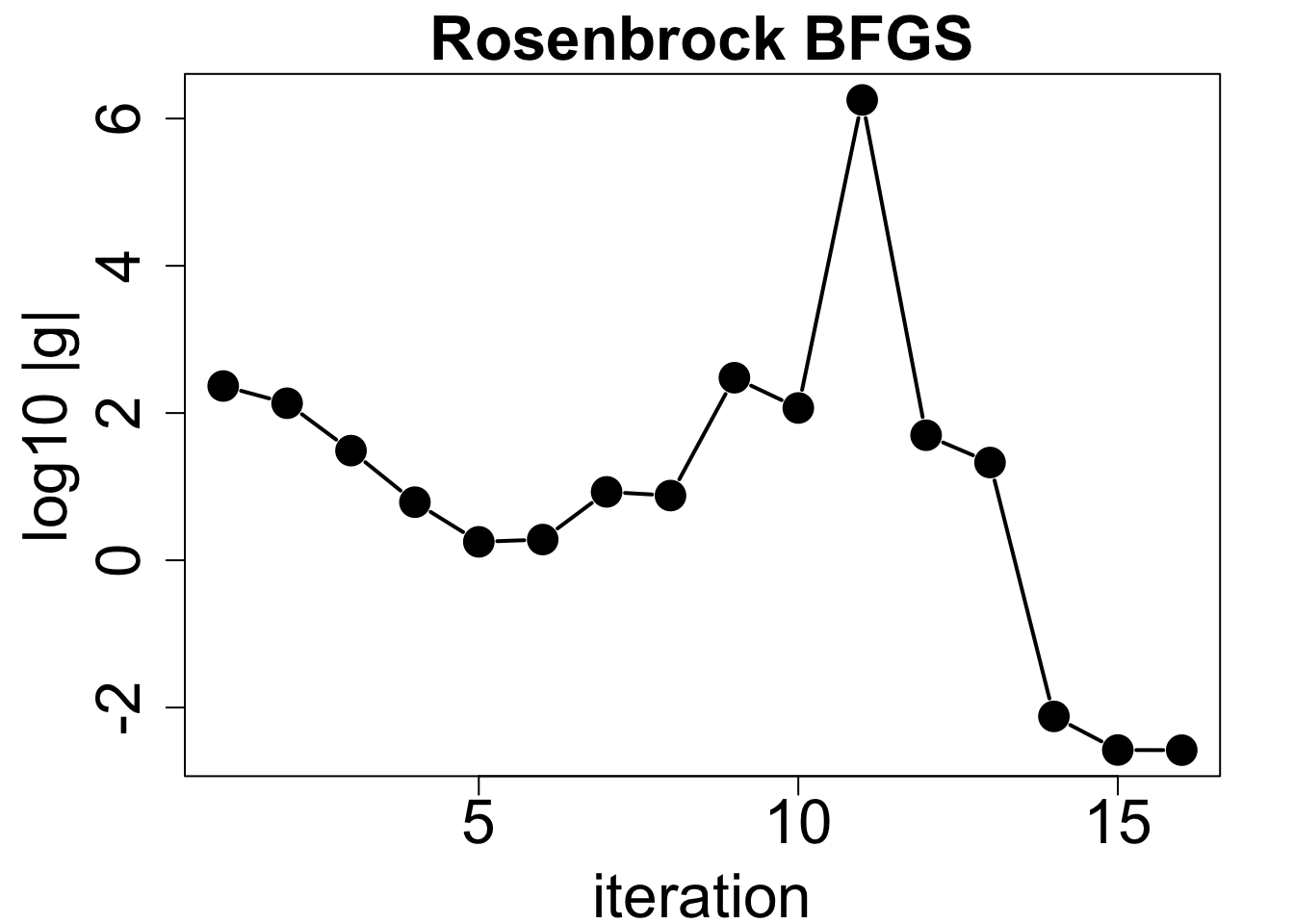
収束はしておらず、コストの変化が小さくなったために打ち切られている。
result$convergence[1] 1次に、Rosenbrock函数の等高線を描画し、最適化の経路を重ねてみる。
xax <- seq(-2, 2, length.out=1001)
yax <- seq(0, 2, length.out=1001)
z <- outer(xax, yax, rosen)
loglevs <- c(1, 3, 10, 30, 100, 300, 1000, 3000, 10000)
contour(xax, yax, z, levels=loglevs, xlab="x", ylab="y",
        main="Rosenbrock BFGS", lwd=2,
        labcex=2, cex.main=2, cex.axis=2, cex.lab=2)
points(result$par[, 1], result$par[, 2], pch=19, cex=2)
lines(result$par[, 1], result$par[, 2], lwd=3)
text(result$par[, 1], result$par[, 2], 1:length(result$cost), pos=c(1, 1, 4), offset=1, cex=2)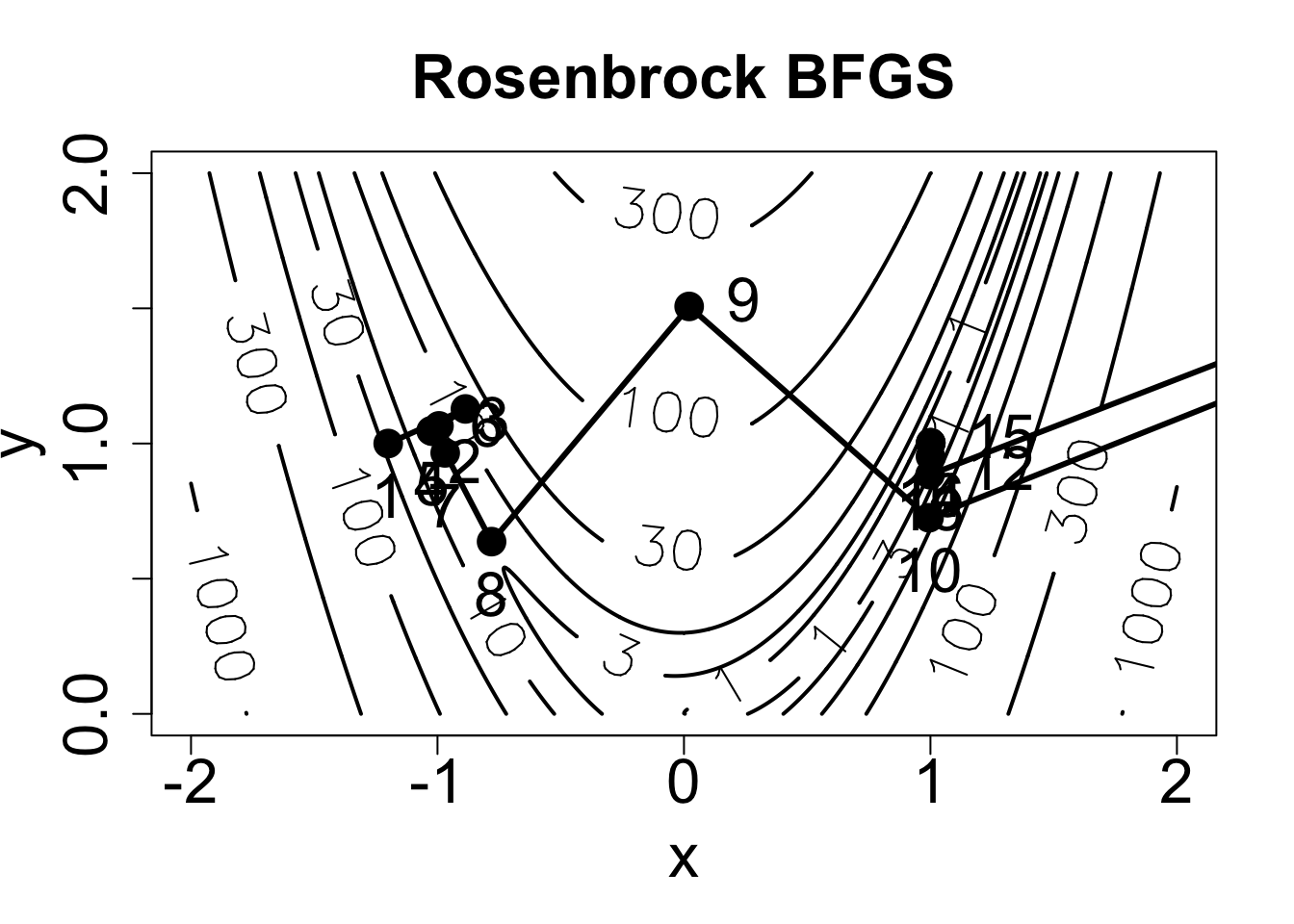
線型探索をしていないので、コストは単調減少ではない。 8〜9ステップ目で勾配を登ることにより、最小値\(x=1\)のある\(x>0\)側に移動している。
References
Broyden, C. G., 1970: The convergence of a class of double-rank minimization algorithms 1. General considerations. IMA J. Appl. Math., 6, 76–90, https://doi.org/10.1093/imamat/6.1.76.
Fletcher, R., 1970: A new approach to variable metric algorithms. The Computer Journal, 13, 317–322, https://doi.org/10.1093/comjnl/13.3.317.
Goldfarb, D., 1970: A family of variable-metric methods derived by variational means. Math. Comput., 24, 23–26, https://doi.org/10.1090/S0025-5718-1970-0258249-6.
Nocedal, J., and Stephen J. Wright, 2006: Numerical Optimization. 2nd ed. Springer,.
Shanno, D. F., 1970: Conditioning of quasi-Newton methods for function minimization. Math. Comput., 24, 647–656, https://doi.org/10.1090/S0025-5718-1970-0274029-X.